Bayesianism vs Frequentism

In recent times the popularity of Bayesian statistics has greatly increased, thanks to the large computing power of modern computers. As a result, there is an ongoing debate on whether the Bayesian or frequentist approach is more suitable for statistical and scientific purposes. A great number of introductory papers on these two schools of statistical inference are available online, therefore I will not spend time reiterating the basic definitions here (for those who are interested I recommend these two documents, which contain excellent introductions to the topic). Instead, my goal is to take a look at which of these two approaches is worth following in order to reach the right statistical conclusions – whatever the definition of ‘right’ may be.

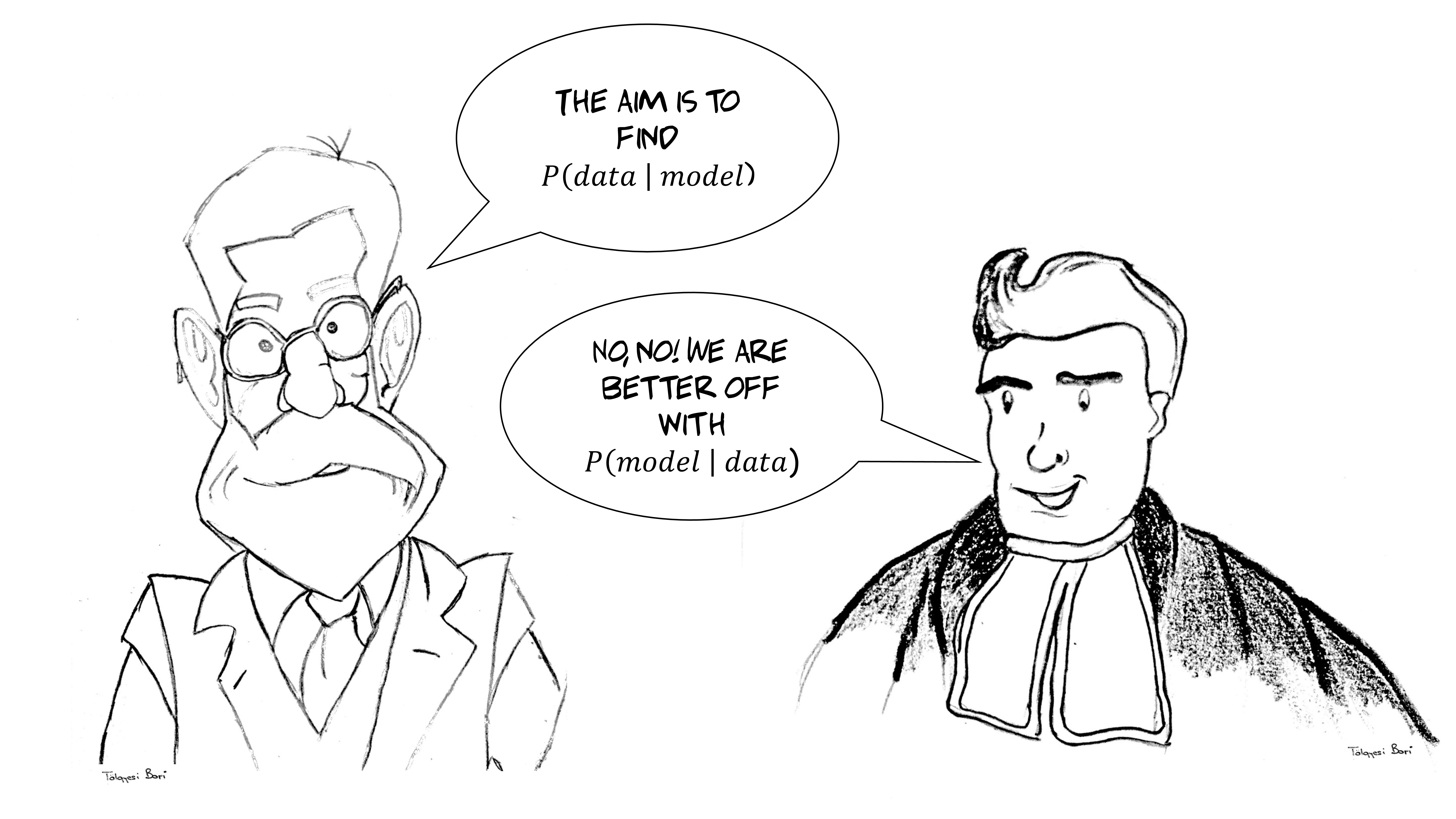
In the Bayesian approach we are looking for the probability P(model|data), which could be translated to our “assuming” the model and “having” the data. That is, our model is uncertain, while the data is our ground truth – the only certain thing we know about reality. In contrast, when we follow the frequentist approach, we are looking for the probability P(data|model), which means that we “assume” the data and “have” the model. In other words, we are certain about our model (at least for working purposes) and we have uncertain measurements, i.e. the data, which may or may not perfectly reflect our model (or even reality).

Null-hypothesis is one hypothesis

At this point, you might easily think that the Bayesian approach makes more sense since we cannot in general know the exact the distribution of a variable inside a population (i.e. the model); you might say we can only know for sure what we observe through the data that we collect. That’s a good point but be aware that a small number of observations can be misleading (i.e. outliers, extremes, noisy measurements and so on). And although we may have observed some data for sure, most of the time we are not interested in the actual data but in the asymptotic inference that we can safely make based on it.

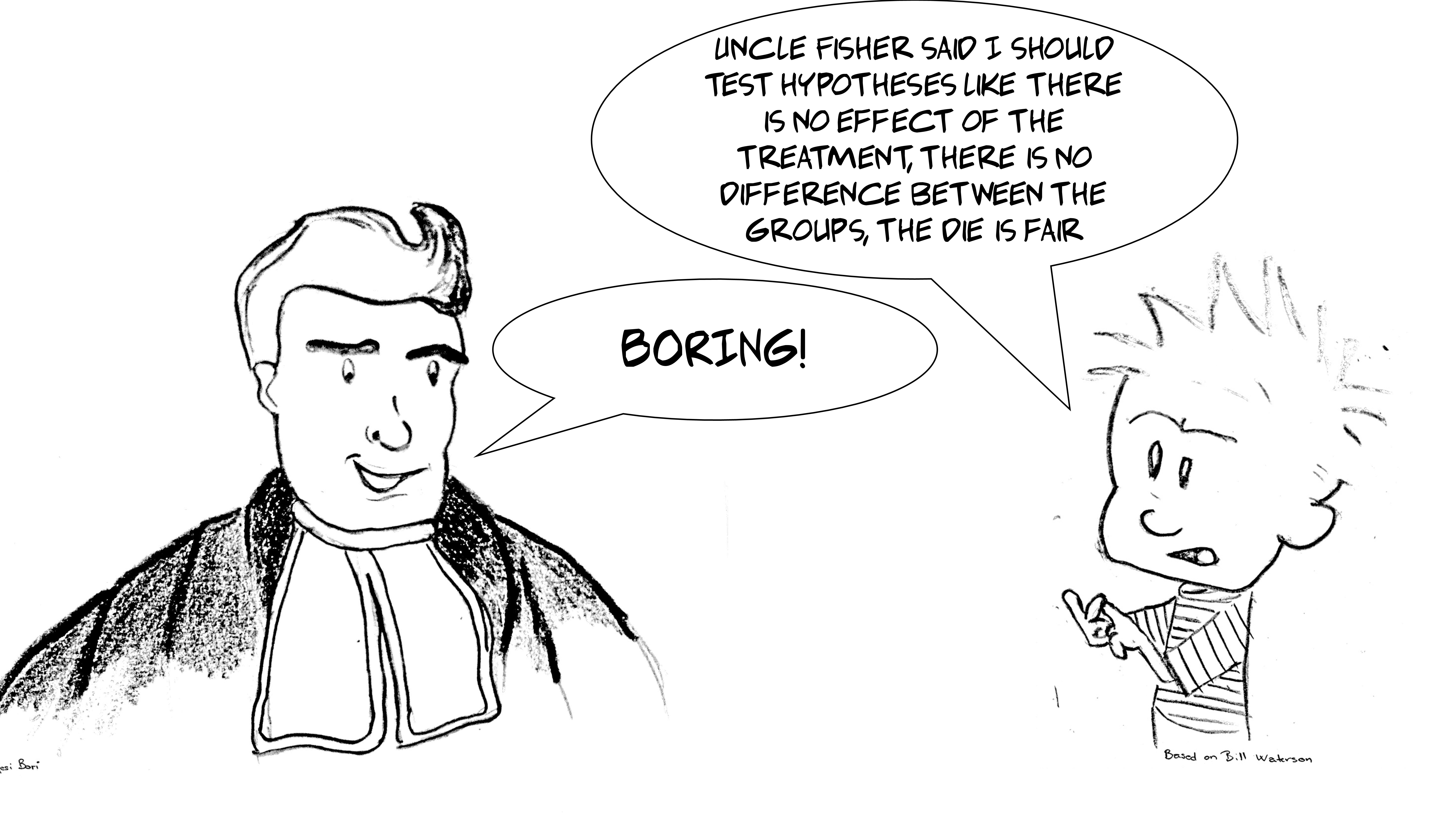
This is why the proponents of frequentist statistics approach the problem by saying: “ok, it’s true that based on our data, we cannot describe the particular population at a satisfactory level of accuracy. However, we can invent a hypothetical population and test how likely it is that our observed data was obtained from that particular population.” Then they would continue; “Of course, the model that we claim is not an elaborate one but it certainly has well-described characteristics (after all we made it)”. This special population model is called the null hypothesis. Most of the time it states something like:

• two groups are from the same population,
• treatment X has no effect,
• this coin or die is fair, etc.

Boring stuff I know but all of this is very handy since we can always reject the null hypothesis, gaining the chance to formulate more interesting conjectures.

And although at first glance you might say that frequentists seem to be a little bit unambitious – seeing as they only talk about what the observed phenomenon is not, instead of what it really is - it’s still the case that statistical methods are used to make grand claims all the time. Statistics has great power and as you know with great power there must also come great responsibility. Statistics can easily lead to false conclusions if not applied with the utmost care, so one is always well advised to tread carefully when it comes to statistics (For those who are interested in how dangerous statistics really is ).

Statistical belief

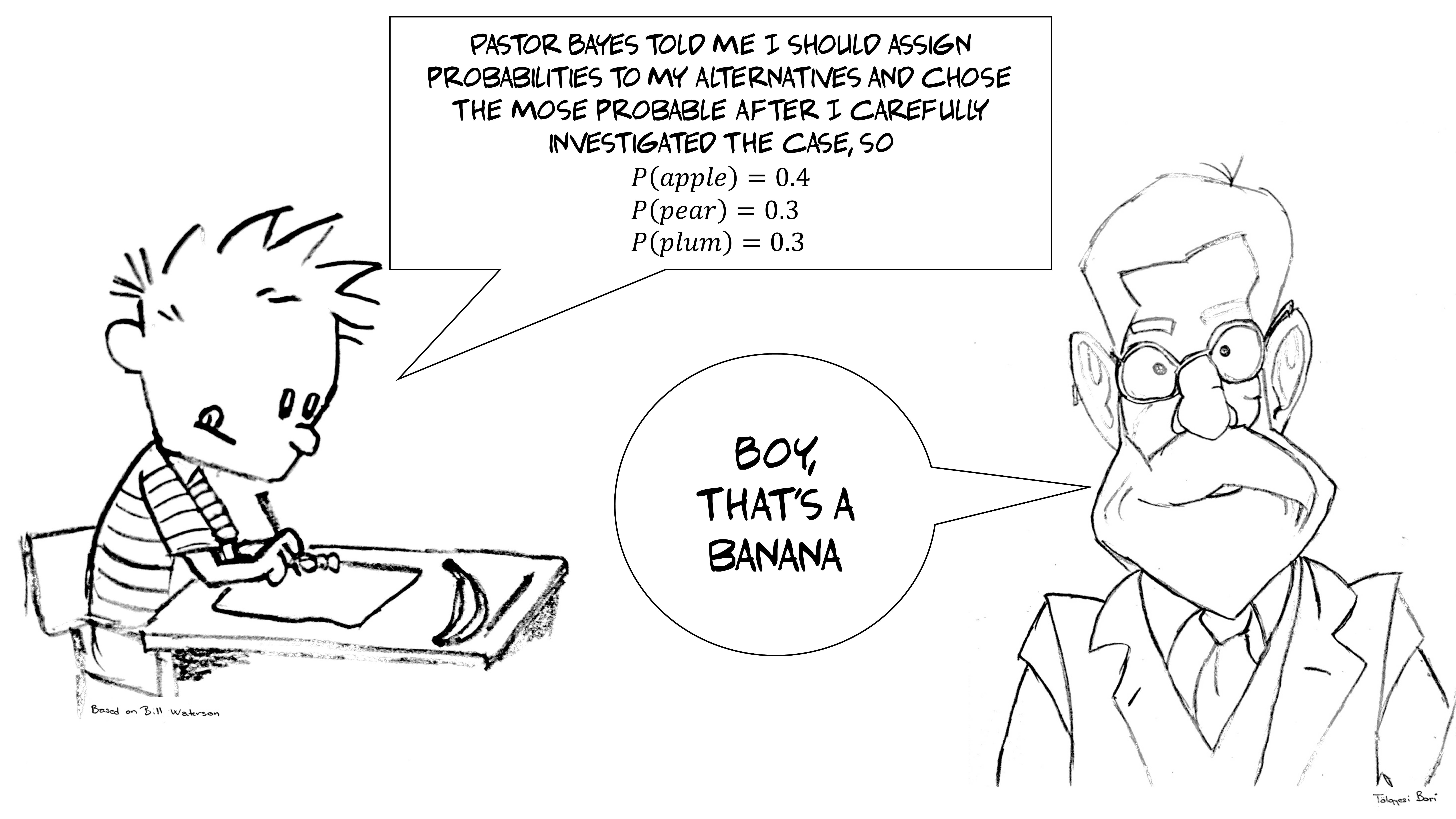
So how about the Bayesian approach? It might be tempting to claim that it is more intuitive and ambitious but some would still argue that the situation is a bit more complex than that. Although Bayesians do come up with a particular hypothesis (e.g. “this medicine will cure the disease”), they often test it in a way such that cases supporting it are implicitly treated as being somewhat more important than cases not supporting it. In other words, the Bayes method speculates that people make hypotheses, expect certain outcomes and compare the real outcomes with those expectations… so one should not pretend that the shape of the prior and the interpretation of data (even the decision to stop collecting data and announce a winning hypothesis) cannot in any way be biased.

In some cases, the Bayesian approach can work quite well as we come up with a limited set of candidate models and distribute the probability between them. Let’s take a look at a Sherlock Holmes-like example here, after all he was one of the key figures of Bayesian hypothesis testing.

Imagine that there was a murder and the murderer might be

• the victim’s wife,
• the victim’s grown-up son,
• the victim’s mother-in-law,
• the postman, and
• the victim himself (suicide).

Let’s distribute the whole (1.0) probability between them, attributing 0.2 to the wife, the son, and the postman, 0.15 to the husband, and the remaining 0.05 to the mother-in-law, who was least likely to commit the crime due to her old age. Now, let’s go on with this thought experiment. We find out that the postman was out of town therefore he couldn’t have been the murderer. We take away the weight of 0.2 attributed to him and rescale the remaining values so that they sum up to 1.0, because someone on the list must be the murderer. Now, it turns out that the wife and the son were in the supermarket. The husband was left-handed so we can rule him out, too, given that the killer was shown by the forensics team to be right-handed. We take away their proportions too, and bamm! We know that the mother-in-law must be guilty of murder.

This could be a nice ending to a TV series, and indeed we often solve practical problems by ruling out possibilities until we are able to hone in on the solution. However, having such a limited number of discrete cases and an easily explorable ground truth is a luxury, something that rarely happens in real life. Imagine, for example, an assassination where we cannot limit the possible suspects to a few people. And that’s not even considering problems where the range of potential solutions is continuous.

The issue here is that if you didn’t even consider the true correct hypothesis to begin with, you might have found evidence for a hypothesis just because no better hypothesis was available. To put this in plain English, if you did not know that Jack the Ripper was also in the house that day, then you might have just locked up a charming 83 year-old grandma without any proof (you Bayesian bastard! :smiley: ). Therefore, by taking some models / hypotheses into consideration but not others (often an infinite number of neglected hypotheses), you will be sure to introduce subjectivity into the investigation.

Mindtwist’n’shout

This is a very important point as we want our statistical methods to yield us the objective truth without us having to rely on our observations at all. Here, the Bayesian statistician is in trouble, because although there is an objective Bayesian method, the strongest ‘weapon’ of the Bayes theorem is indeed the room it leaves for ‘subjectivity’. We like to phrase Bayesian statistics as finding the likelihood of alternatives explaining the data but strictly speaking these alternatives can be driven by prior data, which can be informed, or sensible but rarely objective.

At this point, we could end our discussion here by acknowledging the frequentists as unambitious but objective and the Bayesians as daring but subjective. But come on, let’s not be hypocritical! Humans are prone to disregard information that contradicts their expectations in all sorts of ways (well, not only humans, as illustrated in this funny video with a cat testing the hypothesis of gravity). Indeed, after more than a century of frequentist investigations, researchers still often interpret significant tests as supporting their alternative hypothesis instead of simply not supporting the null hypothesis. If Sir Ronald Fisher (the developer of frequentist statistical methodology) were alive today, such moments would surely make him facepalm.

Of course, we are not entirely wrong making these inferences. After all, we may decide to consider not only the results of a test but also the raw data collected during the test. Furthermore, we sometimes use statistics only to rule out more parsimonious explanations which are covered by the null hypothesis. All the same, one must be aware that the p-value only ever tells us something about the null hypothesis, and that statistical power/confidence/effect size has to be taken into account when making inferences about any alternative hypotheses. Also, tests were developed as mathematical tools to investigate statistical problems but they don’t lead to the correct conclusion all the time. For example, this study shows that if you run A/A tests, after a while there is a high chance that you will find a significant difference between two halves of the sample that is subjected to the same design, even though there is no difference at all in the independent variables

So, as is often the case in real life, the situation is not black and white. In the frequentist approach, we need to specify the expected behaviour of the invented population, specifically informed by the way in which we collected the data. Consider, for example, that you wanted to test your friend’s amazing gift of telling whether milk or tea was poured in the cup first when making the tea the English way (I know, I know, British people are weird, tea+milk??). You set up an experiment of six cups, and she is right in 5 cases and fails only on the last one. Compelling! But is she gifted or was she just lucky?

Following Fisher’s exact test approach: there are 2^6 (=64) possible outcomes in the experiment, and there are 6 different variations among them for failing with one cup only (she could miss the first, the second, etc.). So being right in all but one is extreme but possible even if she responded randomly (6/64 chance). But wait a minute: if you are just guessing you could be right in all of the cases, and that is even more extreme! Therefore, when you decide how unlikely her performance was based on the null-hypothesis of guessing, you should take into account the extremity of her performance and also all the other even more extreme cases, which is then six cases equally extreme like the one observed and one even more extreme where she is right in all the cups when just guessing! This adds up to a p-value of 7/64 (=0.109) for the observed case when the null hypothesis holds. This is not below the 0.05 limit that we consider as the level of significance. Therefore, you could say that your friend’s performance was surprising but it could have been just guessing.

Now, this is the moment when the Bayesian steps up and says:

“You are calling yourself objective, yet you are considering extreme cases which were not observed at all!”

The frequentist could answer:

“These are very strong words. Who said we are just making up these extreme cases? They could have happened in the experiment.”

Indeed, the key word to emphasize is experiment. What if, for example, we decided to collect data until our friend made one mistake? In this case, obtaining the same results we would have assigned a p-value of 0.031 to the data (1/2^5), which is significant. Yet we observed the same data, how could it be that the p-value is different? This is a serious problem since it seems to indicate that the way in which you collect the data defines what cases that are more extreme are possible. But what if you didn’t conduct the experiment but you just have the data?

Well this is tricky for the frequentist, and is partly the reason why frequentists sometimes only go so far as to formulate some very unambitious null-hypotheses. There are rules of thumb which help, though. For example, it is true that the p-value changed a lot in the above case but it is unrealistic to continue an experiment until eternity (i.e. for the p = 0.031 case we assumed the experiment could last forever in the unlikely case of our friend making no errors). Realistic experiments (fixed length, fixed protocol) actually help a lot not only in specifying a null-hypothesis but also in limit the alternatives.

Epilogue

To sum up, let’s draw some conclusions now. We’ve seen that no statistical approach will tell you the truth in every situation, after all statistics is the logic of uncertainty. In every case, we have to include the data and our view of the world in the calculation, and the difference among potential approaches is mostly a question of interpretation.

Bayesian statistics is like a Taylor Swift concert: it’s flashy and trendy, involves much virtuosity (massive calculations) under the hood, and is forward-looking. Frequentist statistics is like spending a night with the Beatles: it can be considered as old-school, uses simple tools, and has a long history. Which approaches you decide to use and in what combination depends on you and the problem. Precisely this last point is where this whole discussion should end up: both approaches were built on our need to be able to make leaps of inference from samples to populations. A long time ago they had different toolsets but today, they are often overlapping (see e.g. permutation, bootstrapping) and complementary.

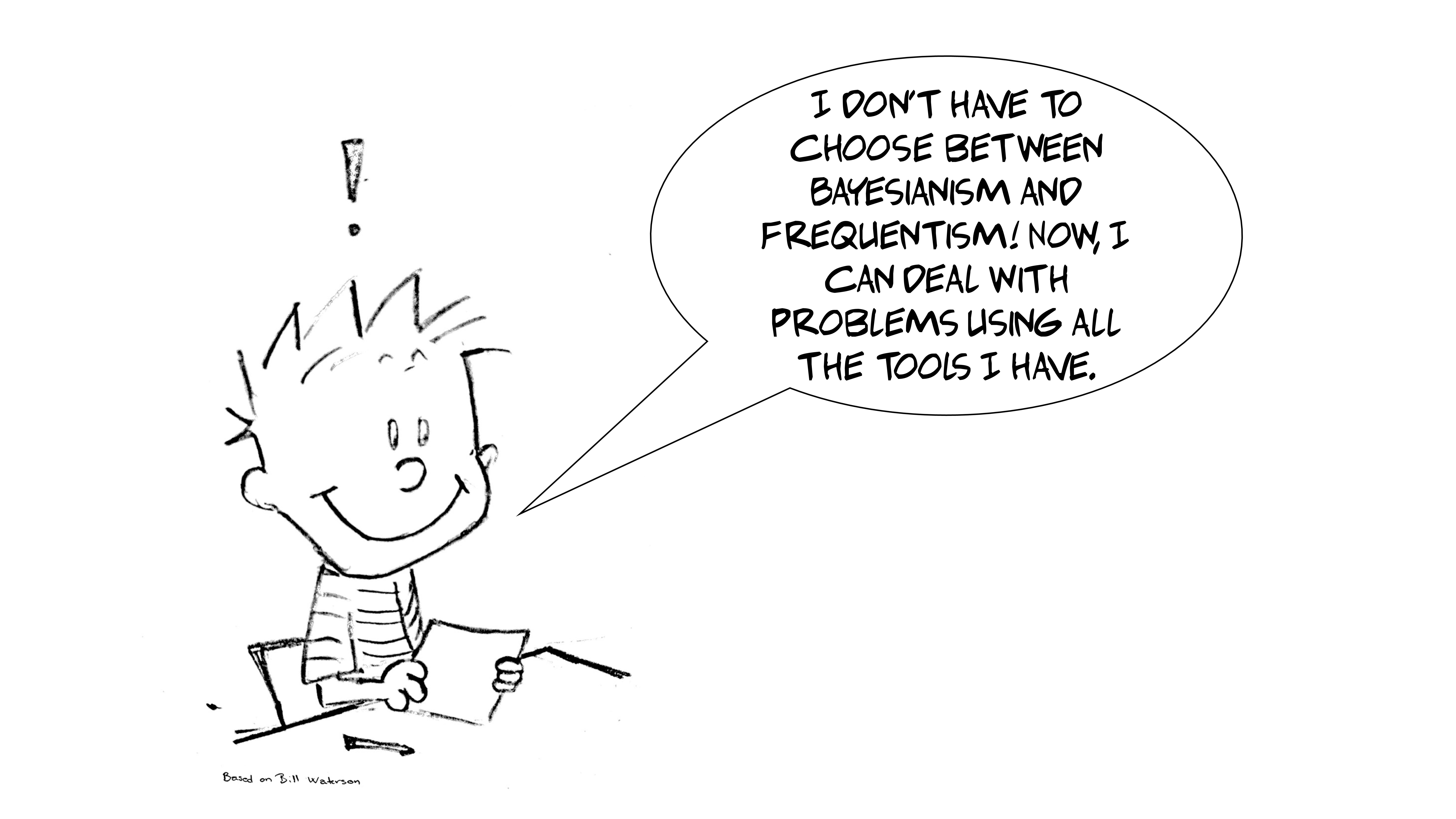
So don’t waste time distinguishing yourself as being either a pure Bayesian or pure frequentist. Instead, solve problems with all the tools you have!

I would like to thank Fanni Kling, Linda Garami PhD, Ádám Csapó PhD, and Daniel Palma for their help in turning the first draft of this post to the current version. Furthermore, I enjoyed the creativity of Borbála Tölgyesi, who provided me with her sketches as illustrations.